It’s true what they say about accountants. We practically live in Microsoft Excel. We learned the basics as part of our collegiate and post-graduate training, but it’s in the workplace at top accounting firms like Weinstein Spira, where we’ve truly honed these skills.
Our team members, Betsy Calvillo, Lee Gyomlai and Travis Aguirre, not only call themselves Excel aficionados, but reign from the millennial population, as well, making them technology whizzes based on their birth years, alone. Each month, Betsy, Lee or Travis will be bringing you, easy-to-learn “hacks” based on questions our clients often ask or positions we often find ourselves in during our work days. These hacks should help you, as well, regardless of what industry you work within.
First up, “center across selection” from Travis and “go to special (F5)” from Lee.
CENTER ACROSS SELECTION (CAS)
Purpose:
CAS and “Merge & Center” are both used for centering data across multiple columns. More importantly, “Center Across Selection” is a fantastic tool for visualization. This hack allows you to showcase and clearly see ownership of certain data, with one header spanning across various columns and their associated data points.
Why use it?
Using CAS allows you to use column selection shortcut keys (ctrl + spacebar) more predictably. Whereas with “Merge & Center,” you’ll often end up selecting more than you intended to with an accidental click of the mouse or space bar, CAS gives you better control over what data remains selected under your new header.
Limitations:
Unfortunately, you can only center across multiple columns with CAS, and not rows. If you’re interested in centering across rows, you would need to do so manually or with “Merge & Center.”
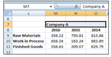
Comparison between CAS and Merge & Center:
Steps for CAS:
1. Select the range that you would like the data to be centered across.
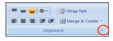
2. Open up the “Format Cells” window (ctrl + 1).
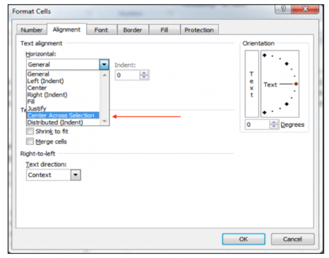
3. On the alignment tab, select “Center Across Selection” from the dropdown menu under “Horizontal.”
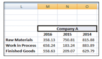
4. The end result should look as follows:
We hope you’ll find this hack as beneficial for organizing and visualizing your data (or your customers’ or clients’ data) as we do. Onto the next hack, Go To Special!
GO TO SPECIAL (F5)
Purpose:
Once you’ve mastered filtering and sorting skills, “Go To Special” is a fantastic tool to add to your arsenal. “Go To Special” allows you to highlight several cells at once, manipulating like data, such as formulas or blank cells, in one easy step.
Why use it?
“Go To Special” is a diverse tool that allows you to manipulate data for a variety of purposes. Including being a time saver, we use it for two practical reasons, but know there are several more ways to benefit from “Go To Special.”
As a precautionary measure – we often use “Go To Special” to select all cells that contain formulas, so as not to accidentally override them when manipulating or moving data later.
To help organize/visualize data – As with “Center Across Selection,” “Go To Special” is a fantastic tool to help you organize data and see things in the best format for your purposes moving forward.
Limitations:
Moving too quickly and not double-checking work could result in errors. As with all your work in Microsoft Excel, it’s important to factor in time to double check work that you’ve done.
Steps and best uses for Go To Special:
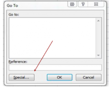
1. Press “F5” to bring up the following menu:
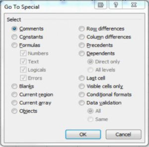
2. Pressing the “Special” button brings up the following options. This menu can be used for several things that are helpful in formatting and save time. For the purposes of this post, we’ll focus on two different ways of utilizing “Go To Special,” “Formulas” and “Blanks.”
Using this menu allows you to highlight a large number of cells at once and then to use one of the buttons above to manipulate your data.
Formulas:
Have you ever received an Excel spreadsheet that needs to be majorly cleaned up and/or organized so that the data, including formulas, clearly makes sense? Utilize this option to determine which cells contain formulas versus which contain hard numbers, following these steps:
- Highlight all data.
- Press “F5”
- Click the “Special” button.
- Choose the “Formulas” button and then hit “OK.”
Excel will then highlight only cells that contain a formula. After this step, you can highlight all of these cells to make changes to formulas only before removing the highlighted areas to make the spreadsheet look like it did beforehand.
Blanks:
To use the “Blanks” function, follow the same four steps as above, but in step four, click the “Blanks” button instead. Choosing blank cells is useful if you want to fill in cells with data that can be scattered or is presented in a difficult-to-use manner.
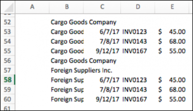
For example, consider the data set within an accounts receivable detail and imagine this repeats for other customers:
The whole column can be selected and then use the “Go To” function to select all the blanks. This will highlight all the blanks. Then follow these steps:
- Press “=” and the up arrow to write a simple formula to grab whatever is in the top cell.
- Press “ctrl” and “enter” to apply that formula to all the selected blank cells.
- Copy the column where the “ctrl” and “enter” formulas and past values were applied.
The result looks like this:
Now, you can filter and delete the unused rows to refine the data as it makes most sense for you. This is a fantastic tool to visualize the representation of data, making it easier to manipulate and allowing you avoid errors.
Let us know if you have success utilizing CAS and F5 in your Excel-related work in the future. We can’t wait to hear about how this helps you save time, avoid mistakes and best understand data.
Be sure to follow Weinstein Spira on Facebook for new Excel hacks each month and share the knowledge with your industry friends and peers.

