Frequent users of Excel are routinely looking for ways to condense an enormous volume of data into useful information. Proficiency with the pivot table feature in Excel can provide a pivotal method by which to encapsulate numbers into what you and your viewers are most interested in.
Purpose
Microsoft Excel’s pivot table functionality allows the user to summarize and sort a mass of information into useful totals in a swift and interactive manner.
Why use it?
The pivot table bypasses time-consuming methods of “sum-if” formulas. It provides instantaneous results for the user, applying averaging, totaling, counting and other calculations to reams of data with various descriptive characteristics.
Limitations
The tables do not automatically update along with modifications in the underlying source data; they need to be refreshed or occasionally recreated altogether. Tables also revert your formatted data (such as currency) into raw numbers, which then require being converted back at your preference.
Example and Steps to Follow:
Your job at Food Mood, a small local grocery, has gone great in your first year, and the company has achieved an impossible growth rate, expanding to six states over that time period. Still, the owner stressed that he needs immediate information to compare and contrast the different locations’ inventory quantities and product types.
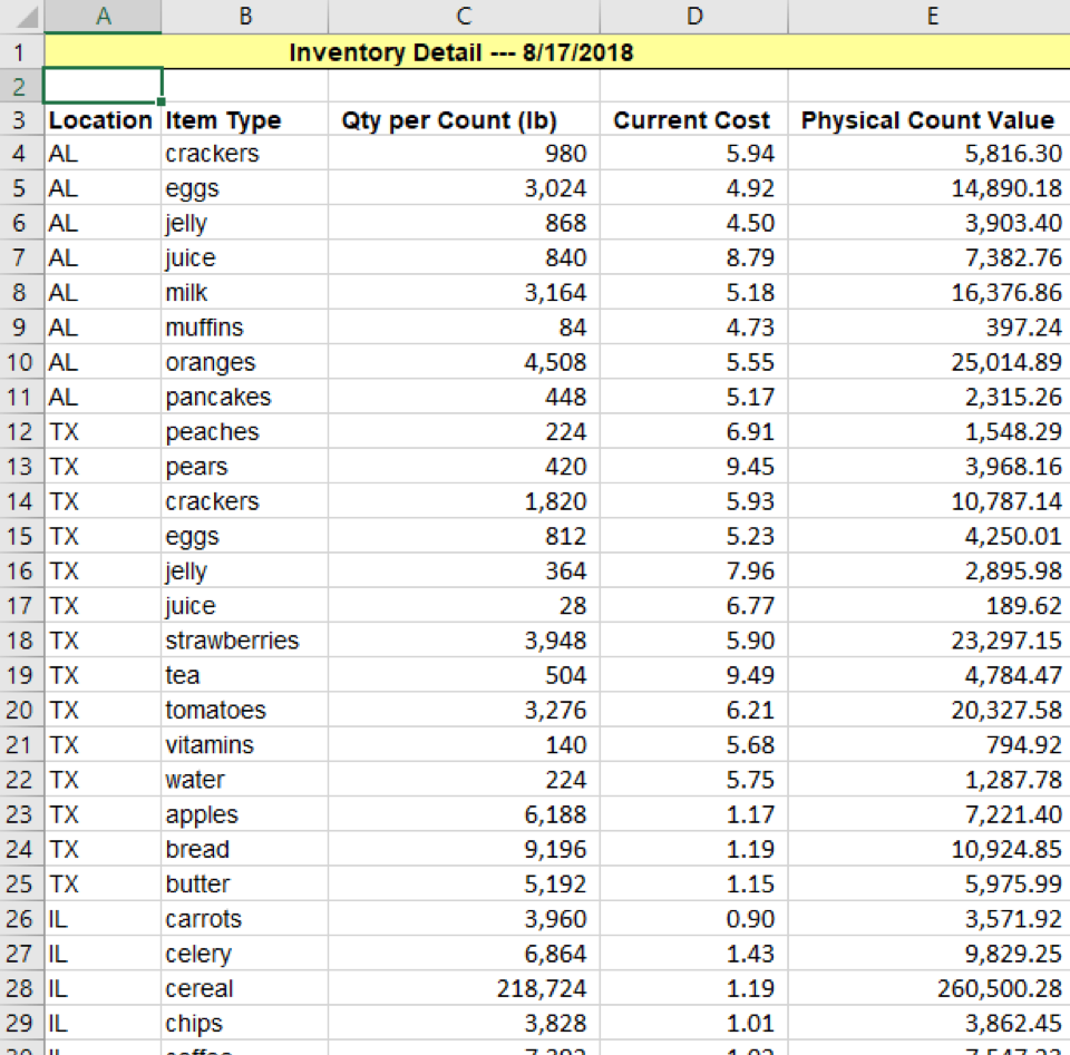
Fortunately, the accounting team working with you at the various locations offers you accurate source data, compiled below, and ready for your crafting.
First, you’d like to understand the relative size of each of the six locations. You sort by location, filter, and then sum the physical count value. Doing this six times… or subtotaling just once can comfortably achieve this result.
However, you’d also like to view the total dollar value of crackers throughout all stores, as well as the total pounds of eggs throughout all stores. So, you change your sorting and filters, each time, achieving the information. So far, you’re getting along all right without a pivot table.
In addition, the owner asks you identify the inventory values of all the types of products throughout all locations in total and sort the products in order of greatest dollar amount, summed for all states in the aggregate. No single sorting routine will accomplish this without considerable time spent manipulating “sum-if” formulas and subtotaling values. After a few more minutes of conversation with the owner, it is obvious that he is looking for customized information which you can most efficiently gather via the pivot table! Set the parameters and watch the magic happen.
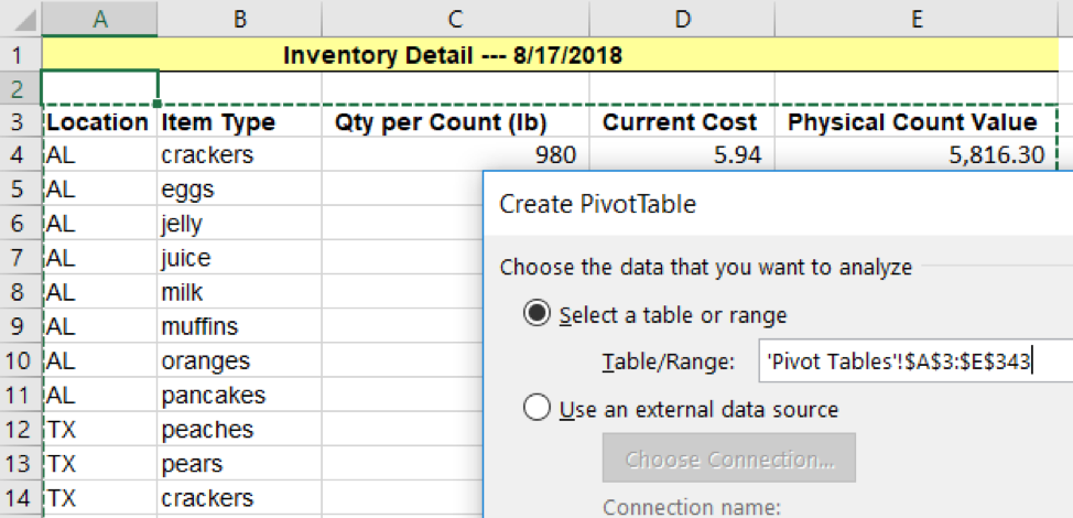
1. Under the “insert” ribbon, click the option for a pivot table. If Excel does not automatically select the range of data you are looking to manipulate, then simply click and drag the cursor to this range:
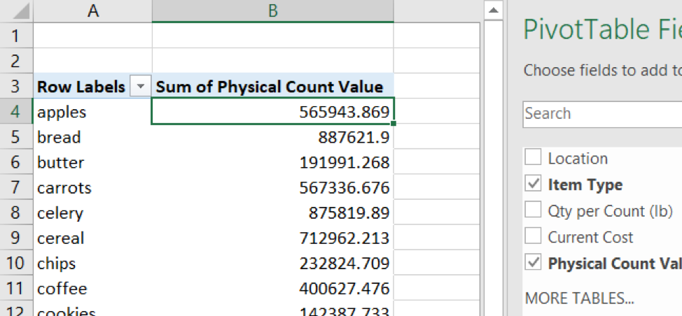
By clicking OK, your fresh and empty pivot table field will generate on a new tab. This is where the customization begins. When the mouse clicked cell is inside the pivot table area, the PivotTable Fields menu will appear on the right of the Excel spreadsheet.
Your boss wants inventory totaled throughout all locations. Two clicks required: Item type and physical count value. Excel will intuitively place them in the correct columns and rows, as it does below. (If it does not, simply drag-and-drop categories from one field to another.)
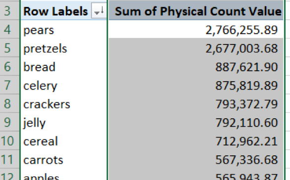
2. Right-click in the cell which you want to sort, to put this by most expensive inventory item.
And with that, you’ve done it! Change the values in column B to number or currency format, and then you can see the totaled inventory across all locations, sorted by value.
The owner looks at the result and says, “I had no clue we had such a high dollar value of pears on hand. It seems a bit excessive. Which location is stocking up on so many pears?”
Another great pivot table tool! Simply double-click on the pears cell, and voila.
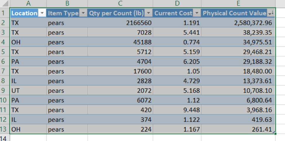
A new tab is opened, with the details comprising the large 2.7 million pears in Texas.
The owner is pleased, and you can continue to utilize this same pivot to respond to his further requests and queries, modifying the parameters of your table by checking and unchecking boxes and dragging fields to customize the resulting table.
Additional items to keep in mind:
- Rather than recreating pivot tables to adjust for altered source data, the tables can simply be refreshed by right-clicking anywhere in the table and selecting “refresh”.
- Pivot tables can be generated on the same tab as the pivot data by selecting a cell’s location in the initial pivot table selection window. Tables can also be moved via standard copy-paste functions.
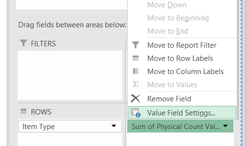
- In this example, we only explored the sum calculation applied to the data. Pivot tables can do much more, such as average and count. To access these, right-click the sum figure as shown below, and click the Value Field Settings
You may also like:


